In part 1 of this blog post I covered the basics of using IO Graphs.  In this post I’ll cover one additional feature: functions.

Functions

There are 6 functions available for use in the IO Graphs:

• SUM(*) – Adds up and plots the value of a field for all instances in the tick interval
• MIN(*) – Plots the minimum value seen for that field in the tick interval
• AVG(*) – Plots the average value seen for that field in the tick interval
• MAX(*) – Plots the maximum value seen for that field in the tick interval
• COUNT(*) – Counts the number of occurrences of the field seen during a tick interval
• LOAD(*) – Used for response time graphs

Let’s look at a few of these functions in action.

Min(), Avg(), and Max() Function Example

For the first example we’ll look at the minimum, average, and maximum times between frames that are sent.  This is useful to see latency between individual frames/packets.  We can combine these functions with the filter ‘frame.time_delta’ to get a visual representation of time between frames and make increases in round trip latency more visible.  If you were looking at a capture that contained multiple conversations between different hosts and wanted to focus on only one pair of hosts you could combine the ‘frame.time_delta’ filter with the source and destination hosts in a filter like ‘ip.addr==x.x.x.x && ip.addr==y.y.y.y’.  I’ll use this in the example below:

Here’s a breakdown of what we did:

• Set the Y-Axis Unit to “Advanced” to make the Calculation fields visible.  If you don’t set this you’ll never see the option to perform calculations.
• The time interval for the x-axis is 1 second, so each bar you see on the graph represents the calculations for that 1 second interval
• Filtered on only the HTTP communication between two specific IP addresses using the filter ‘(ip.addr==192.168.1.4 && ip.addr==128.173.87.169) && http’
• Used three different graphs each with a different calculation – Min(),Avg(), and Max()
• Applied each calculation on the filter criteria ‘frame.time_delta’Set the style to ‘FBar’ because it helps display the data the best
• Set the style to ‘FBar’ because it displays the data nicely

Looking at the graph we can see that at 90 seconds the MAX frame.delta_time for traffic in the capture was almost .7 seconds, which is pretty awful and a result of the latency and packet loss I introduced to this example.  If we wanted to zoom into that specific frame and see what was going on we can just click on the point in the graph and it will jump to that frame in the window in the background, which is frame #1003 in the capture if you are looking at the capture.  This capture had latency and packet loss purposely introduced to exaggerate the types of data you might be able to gather from these graphs but apply to any type of capture you are troubleshooting.  If you see relatively low average times between frames and then a sudden jump at one point in time you can click that frame and narrow in to see what happened at that point in time.

 Count() Function Example

The count() function is useful for graphing some of the TCP analysis flags that we looked at in the first blog post such as retransmissions.  Here’s a sample graph:

Sum() Function Examples

The Sum() function adds up the value of a field.  Two common use cases for this are to look at the amount of TCP data in a capture and to examine TCP sequence numbers.  Let’s look at the TCP length example first.  We’ll setup two graphs, one using the client IP 192.168.1.4 as the source, and the other using the client IP as a destination.  For each graph we will apply the Sum() function with the tcp.len filter. By breaking these out into two different graphs we can see the amount of data traveling in a single direction.

Looking at the graph we can see that the amount of data going towards the client (ip.dst==192.168.1.4 filter) is much higher than the amount of data coming from the client. This is indicated in the red color of the graph.  The black bars show the amount of data traveling from client to server, which is very small in comparison.  This makes sense since the client is simply requesting the file and acknowledging data as it receives it, while the server is sending the large file.  It’s important to note that if you swapped the order of these graphs, putting the client IP as the destination for graph 1 and the client IP as the source in graph 2 that you might not see all of the correct data when using the ‘FBar’ style for both, because the lower the graph number means that graph ends up in the foreground, covering up any higher graph number.

Now let’s look at the TCP sequence number graph for the sample capture that had packet loss and latency.

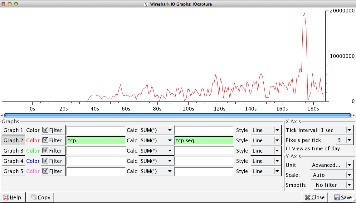
We can see a number of spikes and drops in the graph indicating problems with the TCP transmission.  Let’s compare that to a ‘good’ TCP transfer:

In this capture graph we can see a fairly steady increase in the TCP sequence numbers indicating this transfer was fairly smooth without many retransmissions or lost packets.

Wrap-up

I hope this gave a good overview of the type of advanced graphs you can generate using the built-in Wireshark functions.  The filters shown in this post were some of the more common ones and ones that are highlighted in the excellent Wireshark Network Analysis book by Laura Chappell.  There are a number of other graphs you could use with the functions, it really comes down to understanding how your data transfer should look in an ideal situation and what types of things you know will be missing or different in a ‘bad’ capture.  If you don’t understand the underlying technology like TCP or UDP, it will be difficult to know what to graph and look for when an issue does come up.  Let me know if there are any common filters you use with the IO graph feature, and how they have been useful for you.