X-Forwarded-For, proxies, and IPS

When deploying an IPS appliance I saw a challenge that might come up if you are installing the IPS appliance in addition to a web proxy. One of the by-products of using the default settings of the proxy is that all user traffic going through the proxy ends up being NATted to the IP address of the proxy prior to going to the firewall.  Normally this wouldn’t cause a problem but when you want to setup the IPS appliance to look at all traffic between the inside and firewall it presents an issue.  We lose visibility into what the original client IP address is, all traffic appears as it is coming from one single IP address of the web proxy making IPS logs less useful. In an ideal situation you would be able to place the IPS in a position where it would examine the actual source IP address but not all networks may be able to accommodate this.  One workaround is to utilize the x-forwarded-for header option on your proxy.

X-Forwarded-For Header

There is an industry standard(but not RFC) header available for HTTP called x-forwarded-for, that identifies the originating IP address of an HTTP request, regardless of if it goes through a proxy or load balancer. This header would typically be added by the proxy or load-balancer, but it’s worth noting that there are plugins out there that let a web browser insert this field(whether it is real or spoofed).

Current State

Our current state and traffic flow looks something like this:

before

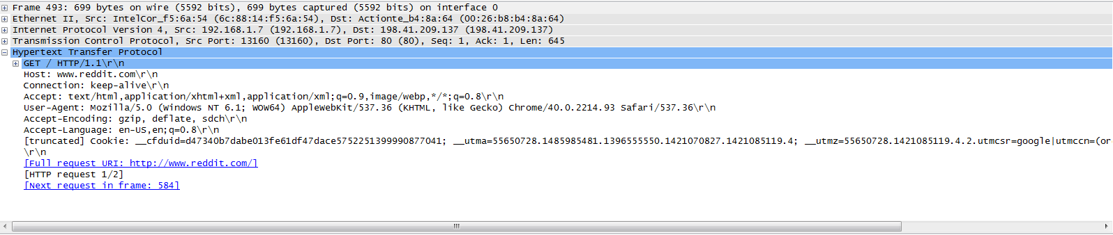
The IP starts as the original ‘real’ client IP, and as it goes through the proxy(websense in this case) it gets changed to the IP of websense.  As it goes through the firewall it then gets changed to the IP of the firewall prior to hitting the Internet. Here’s a screenshot of a HTTP GET in wireshark, without any header:

no xforward

Adding in the header

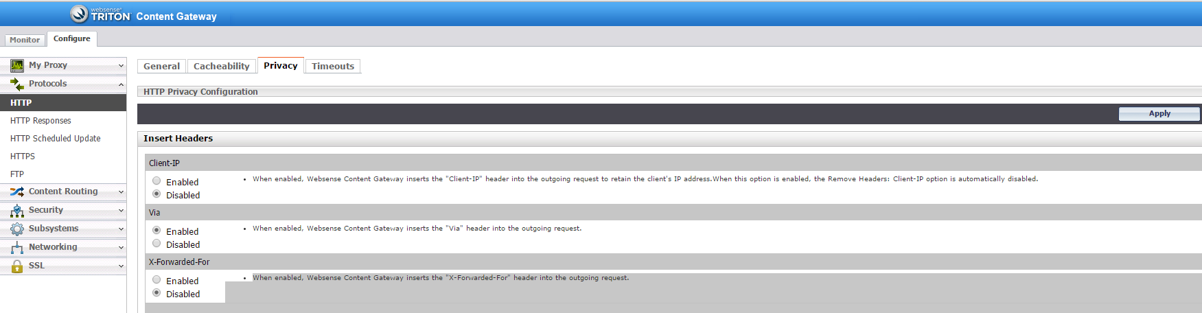
To add the header in Websense you can find the option here in the content gateway GUI:

x-forwarded-for

X-Forwarded State

After enabling the addition of x-forwarded-for headers in Websense this is what our traffic looks like:

After

Here’s a screenshot of an HTTP GET in Wireshark that includes the header, spoofed to 1.2.3.4:

xforward

Inspection

Once this header is added it allows some IPS appliances/software to inspect the x-forwarded-for header and report on the actual client IP address.  Snort currently supports this and there is more detail here. I believe that other IPS appliances such as Cisco’s Sourcefire also supports this option through enabling the HTTP inspect preprocessor and checking ‘Extract Original IP address’ option.  Will work on confirming this and updating the post sometime soon. If you want to look at this traffic in wireshark there is a display filter ‘http.x_forwarded_for’ that will let you filter on x-forwarded-for.

Risks

I’d like to point out that the x-forwarded-for header gets carried in the packet out into the Internet which may or may not concern some people as it releases more information about your internal IP addresses structure than you might have wanted.  I tried to see if there was an ASA feature to strip this header out but couldn’t find anything that looked like it fit besides this Cisco bug report/request for the feature. Also, as mentioned above you can spoof this header pretty easily, it is not authenticated or signed, and is presented in plain text.  Each deployment will be unique and you’ll have to weigh out the risks and whether this is a feature that is worth implementing for your specific environment.

Advertisement

Troubleshooting with Wireshark IO Graphs : Part 2

In part 1 of this blog post I covered the basics of using IO Graphs.  In this post I’ll cover one additional feature: functions.

Functions

There are 6 functions available for use in the IO Graphs:

  • SUM(*) – Adds up and plots the value of a field for all instances in the tick interval
  • MIN(*) – Plots the minimum value seen for that field in the tick interval
  • AVG(*) – Plots the average value seen for that field in the tick interval
  • MAX(*) – Plots the maximum value seen for that field in the tick interval
  • COUNT(*) – Counts the number of occurrences of the field seen during a tick interval
  • LOAD(*) – Used for response time graphs

Let’s look at a few of these functions in action.

Min(), Avg(), and Max() Function Example

For the first example we’ll look at the minimum, average, and maximum times between frames that are sent.  This is useful to see latency between individual frames/packets.  We can combine these functions with the filter ‘frame.time_delta’ to get a visual representation of time between frames and make increases in round trip latency more visible.  If you were looking at a capture that contained multiple conversations between different hosts and wanted to focus on only one pair of hosts you could combine the ‘frame.time_delta’ filter with the source and destination hosts in a filter like ‘ip.addr==x.x.x.x && ip.addr==y.y.y.y’.  I’ll use this in the example below:

Screen Shot 2014-04-13 at 6.23.38 PM

Here’s a breakdown of what we did:

  • Set the Y-Axis Unit to “Advanced” to make the Calculation fields visible.  If you don’t set this you’ll never see the option to perform calculations.
  • The time interval for the x-axis is 1 second, so each bar you see on the graph represents the calculations for that 1 second interval
  • Filtered on only the HTTP communication between two specific IP addresses using the filter ‘(ip.addr==192.168.1.4 && ip.addr==128.173.87.169) && http’
  • Used three different graphs each with a different calculation – Min(),Avg(), and Max()
  • Applied each calculation on the filter criteria ‘frame.time_delta’Set the style to ‘FBar’ because it helps display the data the best
  • Set the style to ‘FBar’ because it displays the data nicely

Looking at the graph we can see that at 90 seconds the MAX frame.delta_time for traffic in the capture was almost .7 seconds, which is pretty awful and a result of the latency and packet loss I introduced to this example.  If we wanted to zoom into that specific frame and see what was going on we can just click on the point in the graph and it will jump to that frame in the window in the background, which is frame #1003 in the capture if you are looking at the capture.  This capture had latency and packet loss purposely introduced to exaggerate the types of data you might be able to gather from these graphs but apply to any type of capture you are troubleshooting.  If you see relatively low average times between frames and then a sudden jump at one point in time you can click that frame and narrow in to see what happened at that point in time.

 Count() Function Example

The count() function is useful for graphing some of the TCP analysis flags that we looked at in the first blog post such as retransmissions.  Here’s a sample graph:

SnipImage

Sum() Function Examples

The Sum() function adds up the value of a field.  Two common use cases for this are to look at the amount of TCP data in a capture and to examine TCP sequence numbers.  Let’s look at the TCP length example first.  We’ll setup two graphs, one using the client IP 192.168.1.4 as the source, and the other using the client IP as a destination.  For each graph we will apply the Sum() function with the tcp.len filter. By breaking these out into two different graphs we can see the amount of data traveling in a single direction.

Screen Shot 2014-04-13 at 8.47.14 PM

Looking at the graph we can see that the amount of data going towards the client (ip.dst==192.168.1.4 filter) is much higher than the amount of data coming from the client. This is indicated in the red color of the graph.  The black bars show the amount of data traveling from client to server, which is very small in comparison.  This makes sense since the client is simply requesting the file and acknowledging data as it receives it, while the server is sending the large file.  It’s important to note that if you swapped the order of these graphs, putting the client IP as the destination for graph 1 and the client IP as the source in graph 2 that you might not see all of the correct data when using the ‘FBar’ style for both, because the lower the graph number means that graph ends up in the foreground, covering up any higher graph number.

Now let’s look at the TCP sequence number graph for the sample capture that had packet loss and latency.

Screen Shot 2014-04-13 at 9.20.16 PM


We can see a number of spikes and drops in the graph indicating problems with the TCP transmission.  Let’s compare that to a ‘good’ TCP transfer:

Screen Shot 2014-04-13 at 9.19.21 PM

In this capture graph we can see a fairly steady increase in the TCP sequence numbers indicating this transfer was fairly smooth without many retransmissions or lost packets.

Wrap-up

I hope this gave a good overview of the type of advanced graphs you can generate using the built-in Wireshark functions.  The filters shown in this post were some of the more common ones and ones that are highlighted in the excellent Wireshark Network Analysis book by Laura Chappell.  There are a number of other graphs you could use with the functions, it really comes down to understanding how your data transfer should look in an ideal situation and what types of things you know will be missing or different in a ‘bad’ capture.  If you don’t understand the underlying technology like TCP or UDP, it will be difficult to know what to graph and look for when an issue does come up.  Let me know if there are any common filters you use with the IO graph feature, and how they have been useful for you.

NAT logging

Recently had a cutover where we copied a basic NAT configuration from one router to a new one.  The configuration was very straight forward, similar to the below:

access-list 3 permit any log

ip nat inside source list 3 interface Loopback2 overload

During the cutover I wasn’t seeing any NAT translations building. Reviewed the config, seemed straight forward. Inside interface defined, outside interface defined, access list and an interface to overload.  After staring at it for awhile I noticed that the ACL had the ‘log’ statement on the permit statement.  Something told me this might be causing the issue. I removed the ‘log’ keyword off the ACL and the translations built immediately.

So what happened – what’s the big deal about logging the matching hits for the NAT ACL? When you put the ‘log’ keyword on an ACL it makes the router process switch that traffic. When you process switch the traffic, NAT does not handle the traffic.  This is well documented in this Cisco FAQ: http://www.cisco.com/c/en/us/support/docs/ip/network-address-translation-nat/26704-nat-faq-00.html

I’m still not sure how this config worked on the old router, I still need to look at the entire config further as there were some other differences(IOS version, IPS enabled, and some others) but its clear that you definitely shouldn’t use the log statement on your NAT ACL’s.

Work smarter, not harder : Excel Concatenate

As a network engineer there’s often times when you need to deal with repetitive tasks such as creating configurations for network devices at multiple sites.  Usually these configs are based on some template, with only minor differences such as IP addresses.  If there are only one or two sites it isn’t bad to create these configurations manually, but if its 10 sites, 20 sites or, hundreds of sites it becomes much worse.  While there a number of different tools or scripts you can program to create these configs, one of the simplest that almost everyone has is Microsoft Excel.

The Functions

Concatenate()

The concatenate function in Excel allows you to take a number of different cells and/or strings of text and concatenate them together.  For example:

=Concatenate(“This is “,”an example”)

Will generate the text “This is an example”. Not the best way to use the function.  A better way would be to refer to cells in the function.

For example, this function:

produces this output, pulling the values from cells ‘A1’ and ‘B1’ and combining them with text

Char()

The Char() function in Excel returns a character based on the Ascii value.  You can pass any ASCII value to the function and it will output the corresponding character.  The main one we are interested in is the “New Line” character.  When we use this in combination with Concatenate() we can put text on different lines.  We can generate this by using ‘CHAR(10)’.

Here’s an example:

will produce this output:

char-ex2

Note: In order for Excel to display the text on different lines you would need to highlight the cell and click the wraptext button.

Building Network Configlets

Now that you understand the basic function we can apply it to networking.  Let’s say you have a spreadsheet listing the various office subnets in 10 different states.  The network was designed so each subnet is a /27 in size with a mask of 255.255.255.224.

spreadsheet

Each site will need it’s own BGP configuration with a unique AS number and advertising all of the subnets at that site.  One way to do this would be to do it manually. Another would be to use the concatenate function in Excel.  Let’s say the config you want to create looks like this:

router bgp <as>

network <wired_network> mask 255.255.255.224

network <wireless_network> mask 255.255.255.224

network <voip_network> mask 255.255.255.224

Using the concatenate() and char() functions we can generate a config per site in only a couple of minutes. This function: concatnetwork-ex1generates this configlet: concatnetwork-ex2

The funtion can now be copied down to the other rows to quickly generate the rest of the sites BGP config:

concatnetwork-ex3

Exporting the Configlets

The last step in the process is to get the configlets from Excel into a text editor or straight into the Cisco CLI.  If you try and copy and paste the cell you used the concatenate function in you will wind up with all of the text between two double quotes.  Since the cell contains the function itself, you can’t double click the cell and copy the text itself.  There are two ways I’ve found to deal with this.

Option 1

One option is to click on the cells you want to copy and paste them into a text editor like Notepad++.  This will give you each configlet surrounded by double quotes.  You can then do something simple like find/replace the double quote with nothing.  See below for a Notepad++ example of this:

notepadplusplus

Option 2

For option 2 you can select the entire column containing the concatenate function outputs and paste them into another column, using the “Paste Special – values only” option.  Once pasted, this will allow you to select and copy / paste the text within the cell(not the cell itself) directly into the CLI without quotes.

paste special

Conclusion

This was one example of how to use Excel to make building multiple configs easier.  It helps to reduce human error as well as decrease the amount of time spent manually building configs.  Other use cases I’ve found for this are building Access List Entries.  It may take some time to get the fields you want to work with in Excel, but once they are in there it becomes a very powerful tool.

Microburst Detection with Wireshark

I recently ran into an issue that was new to me, but after some further research proved to be fairly well known phenomenon that can be difficult to track down. We had a Cisco linecard with some servers connected to it that were generating a fairly large number of output drops on an interface, while at the same time having a low average traffic utilization.  Enter the microburst.

Microbursts are patterns or spikes of traffic that take place in a relatively short time interval(generally sub-second) causing network interfaces to temporarily become oversubscribed and drop traffic. While bursty traffic is fairly common in networks and in most cases is handled by buffers, in some cases the spike in traffic is more than the buffer and interface can handle.  In general, traffic will be more bursty on edge and aggregation links than on core links.

Admitting you have a problem

One of the biggest challenges of microbursts is that you may not even know they are occurring.  Typical monitoring systems(Solarwinds,Cacti,etc) pull interface traffic statistics every one or five minutes by default.  In most cases this gives you a good view into what is going on in your network on the interface level for any traffic patterns that are relatively consistent.  Unfortunately this doesn’t allow you to see bursty traffic that occurs in any short time interval less than the one you are graphing.

Since it isn’t practical to change your monitoring systems to poll interfaces every second, the first place you might notice you are experiencing bursty traffic is in the interface statistics on your switch under “Total Output Drops”. In the output below, we are seeing output drops even though the 5 minute output rate is ~2.9Mbps (much less than the 10Mbps the interface supports).

Switch#sh int fa0/1 | include duplex|output drops|rate
  Full-duplex, 10Mb/s, media type is 10/100BaseTX
  Input queue: 0/75/0/0 (size/max/drops/flushes); Total output drops: 7228
  5 minute input rate 0 bits/sec, 0 packets/sec
5 minute output rate 2921000 bits/sec, 477 packets/sec


Output drops are caused by congested interfaces.  If you are consistently seeing output drops increment in combination with reaching the line speed of the interface your best option is to look into increasing the speed of that link.  In this case you would most likely see this high traffic utilization on a graph.  If you are seeing output drops increment, but the overall traffic utilization of that interface is otherwise low, you are most likely experiencing some type of bursty traffic. One quick change you can make to the interface is to shorten the load interval from the default 5 minutes to 30 seconds using the interface-level command ‘load-interval 30’.  This will change the statistics shown in the output above to report over a 30 second interval instead of 5 minutes and may make the bursty traffic easier to see.  There’s a chance that even 30 seconds may be too long, and if that is the case we can use the Wireshark to look for these bursts.

Using Wireshark to identify the bursty traffic

I setup a simple test in the lab to show what this looks like in practice.  I have a client and server connected to the same Cisco 2960 switch, with the client connected to a 100Mbps port and a server connected to a 10Mbps port. Horribly designed network, and most likely would not be seen in production, but will work to prove the point. The client is sending a consistent 3Mbps stream of traffic to the server using iperf for 5 minutes.  Approximately 60 seconds into the test I start an additional iperf instance and send an additional 10 Mbps to the server for 1 second.  For that 1 second interval the total traffic going to the server is ~13Mbps, greater than it’s max speed of 10Mbps.
While running the tests I used SNMP to poll the interface every 1 minute to see what type of traffic speeds were being reported
throughputgraph
From the graph you can see that it consistently shows ~ 3Mbps of traffic for the entire 5 minute test window. If you were recording data in 1 minute intervals with Solarwinds or Cacti, everything would appear fine with this interface. We don’t see the spike of traffic to 14Mbps that occurs at 1 minute.
I setup a span port on the server port and sent all the traffic to another port with a Wireshark laptop setup.  Start your capture and let it run long enough to capture the suspected burst event (if the output drops seem to increase at the same time each day this may help you in narrowing in on the issue).  Once your capture is done open it up in Wireshark.  The feature we want to use is the “IO Graph”. You can get there via “Statistics” -> “IO Graph”
Wireshark IOGraph

Wireshark IOGraph

Next we need to look at our X and Y Axis values.  By default the X Axis is set to a “Tick Interval” of 1 second.  In my case 1 second is a short enough interval to see the burst of traffic. If your spike in traffic is less then 1 second (millisecond for example), you may need to change the Tick Interval to something less than 1 second like .01 or .001 seconds. The shorter the time interval you choose, the more granular of a view you will have. Change the “Y-Axis” Unit from the default “Packets/Tick” to “Bits/Tick” because that is the unit the interface is reporting.  It immediately becomes obvious on the graph that we do have a spike in traffic, right around the 60 second mark.
IOGraph Burst
In my case the only traffic being sent was test iPerf traffic, but in a real network you would likely have a number of different hosts communicating.  Wireshark will let you click on any point in the graph to view the corresponding packet in the capture  If you click on the top of the spike in the graph,  the main Wireshark window will jump to that packet. Once you identify the hosts causing the burst you can do some further research into what application(s) are causing the spike and continue your troubleshooting.

Conclusion

Identifying microbursts or any bursty traffic is a good example of why it’s important to ‘know what you don’t know’.  If someone complains about seeing issues on a link it’s important not to immediately dismiss the complaint and do some due diligence.  While monitoring interface statistics via SNMP in 1 or 5 minute intervals is an excellent start, it’s important to know that there may be things going on in the network that aren’t showing up in those graphs.  By utilizing a number of different tools you can trace down problems. Reducing the interface load-interval to 30 seconds and tracking your output drops is a good start.Using Wireshark allows you to dive further into the problem and figure out what traffic is causing or contributing to the drops.