Managing Packet Captures

Posted by joekukis

Packet captures are an important part of the network engineers toolkit. They provide a look into what is really going on in your network and help get to the bottom of troubleshooting an issue very quickly. In addition to getting to the bottom of a problem, they also serve as a great learning tool to get a better understanding of how different protocols work, and more importantly how they work in your network. A company called QA cafe has a really great product called Cloudshark, that allows you to manage and analyze your packet captures without installing any software like Wireshark locally. Everything is handled in the web browser. I wanted to write a quick post to take a look at the available options from Cloudshark and how they might work best for you.

Overview

Cloudshark was intended to be used as a hardware or VM appliance within a company. Employees could then upload packet captures to the appliance for storage and analysis. They currently offer a Solo, Professional, and Enterprise version, with the biggest difference being the number of accounts you can create on each and an ability to integrate with Active Directory for the enterprise version. I recently setup the enterprise VM appliance and it was extremely quick to get going, requiring barely any input from me. If you aren’t sure if you want to commit to spending money on the product and want to try it out, or need to send someone a packet capture (that doesn’t contain sensitive information) for further review, they do have a page that allows you to upload up to 10MB of a capture, and then will generate a URL you can send off to someone else. I encourage you to check it out here:https://appliance.cloudshark.org/upload/

Features

Cloudshark really worked to get as many features from Wireshark into the web based product, to the point that sometimes you forget that you are working in a web browser. When you first login to the product you are presented with a page that has a list of your currently uploaded files, as well as a place to upload new files, or search for a saved capture. The interface is clean, and easy to find what you’re looking for.

Increase Cisco TFTP speed

Posted by joekukis

I was recently copying a fairly large 400 MB IOS image to one of our ASR routers and it was taking forever via TFTP. I had seen this before but never really took any time to look into it further. I always switched to FTP, the transfer went faster, and I never looked back. This time I decided to go to Wireshark and take a deeper look. In this post I’ll show you why it’s slow and how to improve the speed, but perhaps more importantly, how to get to the bottom of something like this using Wireshark.

Default TFTP Setting

I performed a packet capture on a TFTP session using the default Cisco router and TFTP server settings. It immediately became clear what the issue was. Here is a screenshot as well as a link to part of the capture file on Cloudshark.

The length of each of the frame is ~500 bytes. This was being transferred over Ethernet, which has a max frame size of 1518 bytes. This means we weren’t fully taking advantage of our available frame size. It’d be the equivalent if I told you to empty a swimming pool and you had the option to use a small plastic cup or a 5 gallon bucket for each trip you took to the pool. The 5 gallon bucket would require far less trips back and forth and decrease the total time needed to empty the pool.

According to the RFC for TFTP, TFTP will transfer data in blocks of 512 bytes at a time, which is what we were seeing with our default settings.

Make it faster

So how do we make this go faster? Well, besides using one of the other TCP based alternatives like SCP or FTP, there is an option in IOS available to increase the TFTP blocksize. In my case I am using an ASR router and the option was there. I didn’t look into seeing which other platforms/ IOS versions this is supported in.

The command you are interested in is: ip tftp blocksize <blocksize> In my case I chose to set the blocksize to 1200 bytes because I have the Cisco VPN client installed which changes your MTU size to 1300 bytes and I didn’t want to deal with fragmentation. Here’s a screenshot of the transfer with the updated block size and link to capture on Cloudshark.org.

Confirming the increase

Besides seeing the bigger blocksize in the capture and noticing the speed was faster, let’s back it up with some real data. If you click the Statistics – Summary menu you can see an average rate for each capture.

Here’s the ‘before’ rate with the default block size:

And here is the summary using the increased block size of 1200 bytes:

That’s almost a 2.5 time increase in performance just by changing the block size for TFTP! Depending on your MTU you may be able to increase this even further, above the 1200 bytes I chose for this example.

Wrapup

Hope this was helpful in not only seeing how you can increase the speed of your transfers with TFTP, but also to see how to troubleshoot what causes issues like this and use tools like Wireshark to get to the bottom of it. One thing to note, TFTP is often the go to default for transferring files to routers and switches but depending on your use case there may be other options that are better. If you are using an unreliable link you may be better off going with the TCP based FTP option, or if you need to securely transfer something SCP is a solid bet. It all depends on what your requirements are.

Easily Parse Netdr output

Posted by joekukis

When processing traffic on a 6500, we generally like to see everything done in hardware. The CPU(really two CPU’s, one for Routing and one for Switching) is usually not involved with the traffic forwarding decision, and only really comes into the picture for a select few types of traffic. Some of these include:

Control traffic (STP,CDP,VTP,HSRP, and similar protocols)
Routing Updates
Traffic destined to the switch (SSH,Telnet, SNMP)
ACL entries with ‘log’ on the end of a line
Fragmentation

For a full list please see this page at Cisco.

Netdr Overview

Netdr is a debug tool included with the 6500 platform that allows you to capture traffic going to/from the route processor or switch processor. Unlike other debugs that come with huge warnings of terrible things that could happen if you run them, netdr is generally considered to be safe. You can run it on a switch that already has very high CPU without any additional negative impact. The goal here is to see what type(s) of traffic are hitting the CPU and causing it to be so high, and then ultimately track that traffic down and stop it. There are a number of really good articles written on Cisco’s site and other blogs on how to use netdr to troubleshoot high cpu. Start here, and then use some Googling to fill in the missing pieces. I don’t want to reinvent the wheel here so I’ll leave how to use the tool to some of the other sites out there.

Interpreting the results

What I really wanted to share was this tool I came across on Cisco’s site. Once you use netdr and get the output it can be somewhat overwhelming to look at as well as tedious to sort through all of the results and get a good idea of what traffic is an issue and what traffic is normally hitting the cpu. The typical output looks something like this:

—— dump of incoming inband packet ——-
interface Vl204, routine mistral_process_rx_packet_inlin, timestamp 15:41:28.768
dbus info: src_vlan 0xCC(204), src_indx 0x341(833), len 0x62(98)
bpdu 0, index_dir 0, flood 0, dont_lrn 0, dest_indx 0x380(896)
EE020400 00CC0400 03410000 62080000 00590418 0E000040 00000000 03800000
mistral hdr: req_token 0x0(0), src_index 0x341(833), rx_offset 0x76(118)
requeue 0, obl_pkt 0, vlan 0xCC(204)
destmac 00.14.F1.12.40.00, srcmac 00.14.F1.12.48.00, protocol 0800
protocol ip: version 0x04, hlen 0x05, tos 0xC0, totlen 80, identifier 6476
df 0, mf 0, fo 0, ttl 1, src 10.20.204.3, dst 10.20.204.2, proto 89
layer 3 data: 45C00050 194C0000 0159F31B 0A14CC03 0A14CC02 0205002C
0AFEFE02 000007D0 00000002 00000110 53B4CAAE 00072005
0A2C004F 0AFEFE04 0000FFFF 00000344 00000380 1800

You can scan the output and see that all the pieces of a typical frame and packet are in there, Things like src/dst MAC, src/dst IP, protocol, and some data in hex format that isn’t easily readable. If you need to repeat this for a large number of packets it gets very tedious. I found (stumbled upon) a great tool on Cisco’s site that makes this all much easier.

Netdr Parser

On the Cisco tools site there is a link to the NetDR Parser. When you first get to the page it gives you the option of pasting your output into the window, or uploading a file that contains netdr output. If you have a lot of netdr data to go through I’d recommend you redirect the output to something like a tftp server using ‘show netdr capture l3-data | redirect tftp://a.b.c.d/netdroutput.txt’. That way you don’t need to worry about logging your ssh session or copy/pasting.

Once you get your NetDR output into the tool you click the ‘Parse Data’ button and the tool goes to work. The results page gives you a Top Talkers section similar to Netflow, with the top L2 and L3 talkers. It also has a detailed table where you can expand any of the rows by clicking on them.

This sample above was based on some netdr output I found on another site, it only contains two packets. If you want to see this in an even more familiar format you can click the ‘Convert to PCap’ button which will export a .pcap file for you to open in wireshark for further review.

Now you can use any of the standard tools built into Wireshark to analyze the captured data. I think its great Cisco came up with this tool to help parse the netdr output. Gives the customer more power to initially troubleshoot without needing to jump immediately to TAC for support.

Troubleshooting with Wireshark IO Graphs : Part 1

Posted by joekukis

One of the lesser used functions of Wireshark is it’s ability to graph different data. When troubleshooting a problem using a packet capture the amount of data can be overwhelming. Scrolling through hundreds or thousands of packets trying to follow a conversation or find a problem you don’t know exists can be frustrating. Wireshark comes with a number of built in graphs that help make these issues become much more obvious. In this post I’ll cover IO graphs.

Basic IO Graphs

The basic Wireshark IO graph will show you the overall traffic seen in a capture file, usually in a per second rate (either packets or bytes). By default the X axis will set the tick interval to one second, and the Y axis will be packets per tick. If you prefer to see the bytes or bits per second, just click the “Unit:” dropdown under “Y Axis” and select which one you want to look at. Using our example, we can see the overall rate of traffic for all captured traffic. At the most basic level, this can be useful for seeing spikes ( or dips) in your traffic and taking a closer look into that traffic. To look into the traffic closer, just click any point on the graph and it will focus on that packet in the background packet list window. If you want to get a more granular view of the traffic, just click the ‘Tick interval” dropdown under “X-Axis” and select a smaller time interval. Let’s take a look at the basic components of the IO graph window.

Graphs – There are 5 different graph buttons, allowing you to graph up to 5 different things at one time. Each Graph button is linked to a different color graph (not changeable). We will go into some further examples using multiple graphs in a little bit.
Filters – Each graph can have a filter associated with it. This filter box uses any of the same display filters you would use in the main Wireshark window.
Styles – There are four different styles you can use: Line, Impulse, Fbar, and Dots. If you are graphing multiple items, you might want to choose different styles for each graph to make sure everything is visible and one graph doesn’t cover up another. Graph 1 will always be the foreground layer.
X and Y Axis – Wireshark will automatically define both axis’ based on traffic being plotted. The default for the x axis is 1 second.The X axis default is usually OK for looking at most traffic, but if you are trying to look at bursty traffic you may need to use a smaller X-Axis tick interval. Pixels per tick allows you to alter the spacing of the ticks on the graph. The default for the y axis is packets per tick. Other options include bytes/tick, bits/tick, or Advanced. We’ll touch on the Advanced features later on. The scale is set to auto by default.

Basic Traffic Rate Graph

To start, open up this sample packet capture, or your own in Wireshark and click on Statistics – IO Graphs. This capture is an HTTP download that encountered packet loss. I also have a constant ping going to the host. Let’s stop for a second and just point out the obvious.

The graph color is black because the default graph is Graph 1, and Graph 1 is always tied to the black color
The graph is showing all traffic because the filter box is blank.
The default view will show us packets per second.

While the default view of packets/second is OK, it’s not super useful for most troubleshooting I’ve run into. Let’s change the Y Axis to bits/tick so we can see a traffic rate in bits per second and get a rate of traffic. We can see that the peak of traffic is somewhere around 300kbps. If you had a capture you were looking at that had places where the traffic rate dropped to zero, that might be a reason to dive further into those time periods and see what is going on. This is a case where it would be very easy to spot on the graph, but might not be as obvious just scrolling through the packet list.

Filtering

Each graph allows you to apply a filter to it. There aren’t really any limitations on what you can filter here. Anything that is a display filter is fair game and can help you with your analysis. Let’s start off with something basic. I’ll create two different graphs, one graphing HTTP traffic and one graphing ICMP. We can see Graph 1(Black Line style) is filtered using ‘http’ and Graph 2(Red Fbar style) is filtered using ‘icmp’. You might notice there are some gaps in the red Fbar lines which are filtered on ICMP traffic. Let’s have a closer look at those.

I’ll set up two Graphs, one showing ICMP Echo(Type=8) and one showing ICMP Reply(Type=0). If everything were working correctly I would expect to see a constant stream of replies for every echo request. Let’s see what we have: We can see that the red impulse lines for Graph2(icmp type==0 – ICMP Reply) have gaps and aren’t consistently spread across the graph, while the ICMP requests are pretty consistent across the whole graph. This indicates that some replies were not received. In this example I had introduced packet loss to cause these replies to drop. This is what the ping looked like on the CLI:

Common Troubleshooting Filters

For troubleshooting slow downloads/application issues there are a handful of filters that are especially helpful:

tcp.analysis.lost_segment – Indicates we’ve seen a gap in sequence numbers in the capture. Packet loss can lead to duplicate ACKs, which leads to retransmissions
tcp.analysis.duplicate_ack – displays packets that were acknowledged more than one time. A high number of duplicate ACKs is a sign of possible high latency between TCP endpoints
tcp.analysis.retransmission – Displays all retransmissions in the capture. A few retransmissions are OK, excessive retransmissions are bad. This usually shows up as slow application performance and/or packet loss to the user
tcp.analysis.window_update – this will graph the size of the TCP window throughout your transfer. If you see this window size drop down to zero(or near zero) during your transfer it means the sender has backed off and is waiting for the receiver to acknowledge all of the data already sent. This would indicate the receiving end is overwhelmed.
tcp.analysis.bytes_in_flight – the number of unacknowledged bytes on the wire at a point in time. The number of unacknowledged bytes should never exceed your TCP window size (defined in the initial 3 way TCP handshake) and to maximize your throughput you want to get as close as possible to the TCP window size. If you see a number consistently lower than your TCP window size, it could indicate packet loss or some other issue along the path preventing you from maximizing throughput.
tcp.analysis.ack_rtt – measures the time delta between capturing a TCP packet and the corresponding ACK for that packet. If this time is long it could indicate some type of delay in the network (packet loss, congestion, etc)

Let’s apply a few of these filters to our capture file: In this graph we have 4 things going on:

Graph 1 (Black Line) is the overall traffic filtered on HTTP, being displayed in packets/tick, the tick interval is 1 second so we are looking at packets/second
Graph 2 (Red FBar Style) is the TCP Lost segments
Graph 3 (Green Fbar Style) is the TCP Duplicate Acks
Graph 4 (Blue Fbar Style) is the TCP Retransmissions

From this capture we can see that there are a fairly large number of retransmissions and duplicate ACKs compared to the amount of overall HTTP traffic(black line). Looking at the packet list alone, you may be able to get some idea that there are a number of duplicate acks and retransmissions going on but it’s hard to get a grasp of when they are occurring throughout the capture and in what proportion they occur compared to overall traffic. This graph makes it a little clearer.

In the next post I’m going to go into using some of the more advanced features of IO graphs such as functions and comparing multiple captures in one graph. Hope this was helpful to get you started with IO graphs.

Microburst Detection with Wireshark

Posted by joekukis

I recently ran into an issue that was new to me, but after some further research proved to be fairly well known phenomenon that can be difficult to track down. We had a Cisco linecard with some servers connected to it that were generating a fairly large number of output drops on an interface, while at the same time having a low average traffic utilization. Enter the microburst.

Microbursts are patterns or spikes of traffic that take place in a relatively short time interval(generally sub-second) causing network interfaces to temporarily become oversubscribed and drop traffic. While bursty traffic is fairly common in networks and in most cases is handled by buffers, in some cases the spike in traffic is more than the buffer and interface can handle. In general, traffic will be more bursty on edge and aggregation links than on core links.

Admitting you have a problem

One of the biggest challenges of microbursts is that you may not even know they are occurring. Typical monitoring systems(Solarwinds,Cacti,etc) pull interface traffic statistics every one or five minutes by default. In most cases this gives you a good view into what is going on in your network on the interface level for any traffic patterns that are relatively consistent. Unfortunately this doesn’t allow you to see bursty traffic that occurs in any short time interval less than the one you are graphing.

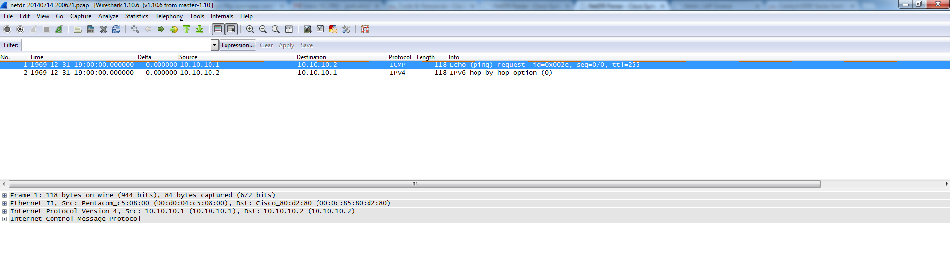
Since it isn’t practical to change your monitoring systems to poll interfaces every second, the first place you might notice you are experiencing bursty traffic is in the interface statistics on your switch under “Total Output Drops”. In the output below, we are seeing output drops even though the 5 minute output rate is ~2.9Mbps (much less than the 10Mbps the interface supports).

Switch#sh int fa0/1 | include duplex|output drops|rate

Full-duplex, 10Mb/s, media type is 10/100BaseTX

Input queue: 0/75/0/0 (size/max/drops/flushes); Total output drops: 7228

5 minute input rate 0 bits/sec, 0 packets/sec

5 minute output rate 2921000 bits/sec, 477 packets/sec

Output drops are caused by congested interfaces. If you are consistently seeing output drops increment in combination with reaching the line speed of the interface your best option is to look into increasing the speed of that link. In this case you would most likely see this high traffic utilization on a graph. If you are seeing output drops increment, but the overall traffic utilization of that interface is otherwise low, you are most likely experiencing some type of bursty traffic. One quick change you can make to the interface is to shorten the load interval from the default 5 minutes to 30 seconds using the interface-level command ‘load-interval 30’. This will change the statistics shown in the output above to report over a 30 second interval instead of 5 minutes and may make the bursty traffic easier to see. There’s a chance that even 30 seconds may be too long, and if that is the case we can use the Wireshark to look for these bursts.

Using Wireshark to identify the bursty traffic

I setup a simple test in the lab to show what this looks like in practice. I have a client and server connected to the same Cisco 2960 switch, with the client connected to a 100Mbps port and a server connected to a 10Mbps port. Horribly designed network, and most likely would not be seen in production, but will work to prove the point. The client is sending a consistent 3Mbps stream of traffic to the server using iperf for 5 minutes. Approximately 60 seconds into the test I start an additional iperf instance and send an additional 10 Mbps to the server for 1 second. For that 1 second interval the total traffic going to the server is ~13Mbps, greater than it’s max speed of 10Mbps.

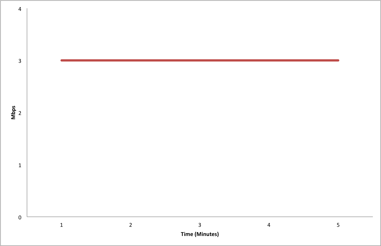
While running the tests I used SNMP to poll the interface every 1 minute to see what type of traffic speeds were being reported

From the graph you can see that it consistently shows ~ 3Mbps of traffic for the entire 5 minute test window. If you were recording data in 1 minute intervals with Solarwinds or Cacti, everything would appear fine with this interface. We don’t see the spike of traffic to 14Mbps that occurs at 1 minute.

I setup a span port on the server port and sent all the traffic to another port with a Wireshark laptop setup. Start your capture and let it run long enough to capture the suspected burst event (if the output drops seem to increase at the same time each day this may help you in narrowing in on the issue). Once your capture is done open it up in Wireshark. The feature we want to use is the “IO Graph”. You can get there via “Statistics” -> “IO Graph”

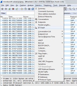
Wireshark IOGraph

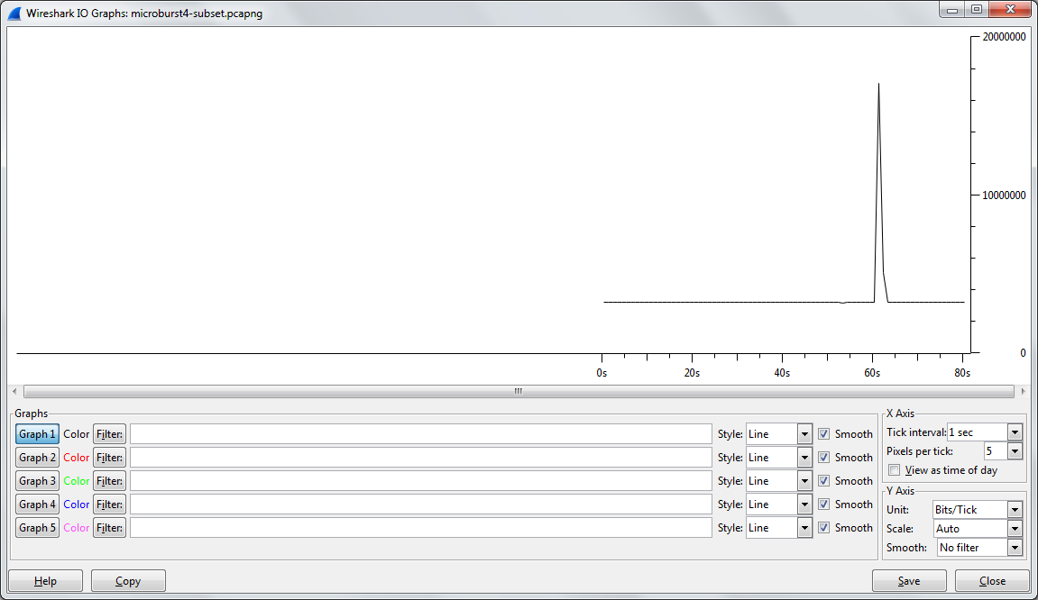
Next we need to look at our X and Y Axis values. By default the X Axis is set to a “Tick Interval” of 1 second. In my case 1 second is a short enough interval to see the burst of traffic. If your spike in traffic is less then 1 second (millisecond for example), you may need to change the Tick Interval to something less than 1 second like .01 or .001 seconds. The shorter the time interval you choose, the more granular of a view you will have. Change the “Y-Axis” Unit from the default “Packets/Tick” to “Bits/Tick” because that is the unit the interface is reporting. It immediately becomes obvious on the graph that we do have a spike in traffic, right around the 60 second mark.

In my case the only traffic being sent was test iPerf traffic, but in a real network you would likely have a number of different hosts communicating. Wireshark will let you click on any point in the graph to view the corresponding packet in the capture If you click on the top of the spike in the graph, the main Wireshark window will jump to that packet. Once you identify the hosts causing the burst you can do some further research into what application(s) are causing the spike and continue your troubleshooting.

Conclusion

Identifying microbursts or any bursty traffic is a good example of why it’s important to ‘know what you don’t know’. If someone complains about seeing issues on a link it’s important not to immediately dismiss the complaint and do some due diligence. While monitoring interface statistics via SNMP in 1 or 5 minute intervals is an excellent start, it’s important to know that there may be things going on in the network that aren’t showing up in those graphs. By utilizing a number of different tools you can trace down problems. Reducing the interface load-interval to 30 seconds and tracking your output drops is a good start.Using Wireshark allows you to dive further into the problem and figure out what traffic is causing or contributing to the drops.