One of the lesser used functions of Wireshark is it’s ability to graph different data. When troubleshooting a problem using a packet capture the amount of data can be overwhelming. Scrolling through hundreds or thousands of packets trying to follow a conversation or find a problem you don’t know exists can be frustrating. Wireshark comes with a number of built in graphs that help make these issues become much more obvious. In this post I’ll cover IO graphs.
Basic IO Graphs
The basic Wireshark IO graph will show you the overall traffic seen in a capture file, usually in a per second rate (either packets or bytes). By default the X axis will set the tick interval to one second, and the Y axis will be packets per tick. If you prefer to see the bytes or bits per second, just click the “Unit:” dropdown under “Y Axis” and select which one you want to look at. Using our example, we can see the overall rate of traffic for all captured traffic. At the most basic level, this can be useful for seeing spikes ( or dips) in your traffic and taking a closer look into that traffic. To look into the traffic closer, just click any point on the graph and it will focus on that packet in the background packet list window. If you want to get a more granular view of the traffic, just click the ‘Tick interval” dropdown under “X-Axis” and select a smaller time interval. Let’s take a look at the basic components of the IO graph window.
- Graphs – There are 5 different graph buttons, allowing you to graph up to 5 different things at one time. Each Graph button is linked to a different color graph (not changeable). We will go into some further examples using multiple graphs in a little bit.
- Filters – Each graph can have a filter associated with it. This filter box uses any of the same display filters you would use in the main Wireshark window.
- Styles – There are four different styles you can use: Line, Impulse, Fbar, and Dots. If you are graphing multiple items, you might want to choose different styles for each graph to make sure everything is visible and one graph doesn’t cover up another. Graph 1 will always be the foreground layer.
- X and Y Axis – Wireshark will automatically define both axis’ based on traffic being plotted. The default for the x axis is 1 second.The X axis default is usually OK for looking at most traffic, but if you are trying to look at bursty traffic you may need to use a smaller X-Axis tick interval. Pixels per tick allows you to alter the spacing of the ticks on the graph. The default for the y axis is packets per tick. Other options include bytes/tick, bits/tick, or Advanced. We’ll touch on the Advanced features later on. The scale is set to auto by default.
Basic Traffic Rate Graph
To start, open up this sample packet capture, or your own in Wireshark and click on Statistics – IO Graphs. This capture is an HTTP download that encountered packet loss. I also have a constant ping going to the host. Let’s stop for a second and just point out the obvious. 
- The graph color is black because the default graph is Graph 1, and Graph 1 is always tied to the black color
- The graph is showing all traffic because the filter box is blank.
- The default view will show us packets per second.
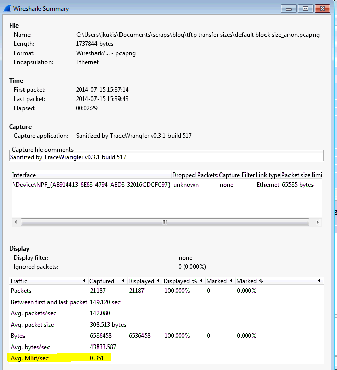
While the default view of packets/second is OK, it’s not super useful for most troubleshooting I’ve run into. Let’s change the Y Axis to bits/tick so we can see a traffic rate in bits per second and get a rate of traffic. We can see that the peak of traffic is somewhere around 300kbps. If you had a capture you were looking at that had places where the traffic rate dropped to zero, that might be a reason to dive further into those time periods and see what is going on. This is a case where it would be very easy to spot on the graph, but might not be as obvious just scrolling through the packet list.
Filtering
Each graph allows you to apply a filter to it. There aren’t really any limitations on what you can filter here. Anything that is a display filter is fair game and can help you with your analysis. Let’s start off with something basic. I’ll create two different graphs, one graphing HTTP traffic and one graphing ICMP. We can see Graph 1(Black Line style) is filtered using ‘http’ and Graph 2(Red Fbar style) is filtered using ‘icmp’. You might notice there are some gaps in the red Fbar lines which are filtered on ICMP traffic. Let’s have a closer look at those.
I’ll set up two Graphs, one showing ICMP Echo(Type=8) and one showing ICMP Reply(Type=0). If everything were working correctly I would expect to see a constant stream of replies for every echo request. Let’s see what we have:  We can see that the red impulse lines for Graph2(icmp type==0 – ICMP Reply) have gaps and aren’t consistently spread across the graph, while the ICMP requests are pretty consistent across the whole graph. This indicates that some replies were not received. In this example I had introduced packet loss to cause these replies to drop. This is what the ping looked like on the CLI:
Common Troubleshooting Filters
For troubleshooting slow downloads/application issues there are a handful of filters that are especially helpful:
- tcp.analysis.lost_segment – Indicates we’ve seen a gap in sequence numbers in the capture. Packet loss can lead to duplicate ACKs, which leads to retransmissions
- tcp.analysis.duplicate_ack – displays packets that were acknowledged more than one time. A high number of duplicate ACKs is a sign of possible high latency between TCP endpoints
- tcp.analysis.retransmission – Displays all retransmissions in the capture. A few retransmissions are OK, excessive retransmissions are bad. This usually shows up as slow application performance and/or packet loss to the user
- tcp.analysis.window_update – this will graph the size of the TCP window throughout your transfer. If you see this window size drop down to zero(or near zero) during your transfer it means the sender has backed off and is waiting for the receiver to acknowledge all of the data already sent. This would indicate the receiving end is overwhelmed.
- tcp.analysis.bytes_in_flight – the number of unacknowledged bytes on the wire at a point in time. The number of unacknowledged bytes should never exceed your TCP window size (defined in the initial 3 way TCP handshake) and to maximize your throughput you want to get as close as possible to the TCP window size. If you see a number consistently lower than your TCP window size, it could indicate packet loss or some other issue along the path preventing you from maximizing throughput.
- tcp.analysis.ack_rtt – measures the time delta between capturing a TCP packet and the corresponding ACK for that packet. If this time is long it could indicate some type of delay in the network (packet loss, congestion, etc)
Let’s apply a few of these filters to our capture file:  In this graph we have 4 things going on:
- Graph 1 (Black Line) is the overall traffic filtered on HTTP, being displayed in packets/tick, the tick interval is 1 second so we are looking at packets/second
- Graph 2 (Red FBar Style) is the TCP Lost segments
- Graph 3 (Green Fbar Style) is the TCP Duplicate Acks
- Graph 4 (Blue Fbar Style) is the TCP Retransmissions
From this capture we can see that there are a fairly large number of retransmissions and duplicate ACKs compared to the amount of overall HTTP traffic(black line). Looking at the packet list alone, you may be able to get some idea that there are a number of duplicate acks and retransmissions going on but it’s hard to get a grasp of when they are occurring throughout the capture and in what proportion they occur compared to overall traffic. This graph makes it a little clearer.
In the next post I’m going to go into using some of the more advanced features of IO graphs such as functions and comparing multiple captures in one graph. Hope this was helpful to get you started with IO graphs.